The 90th academy awards came and went this month. My wife is a bit of an Oscar's fanatic, and she's managed to sweep me up in her mania. We host an Oscars-watching party every year - I tend bar and she makes snacks that are matched up to themes of nominated movies. We also print out ballots for all of the guests and let them nominate their favorites. Whoever gets the most right gets a prize; my wife has won every year for the last three, though, so we're starting to be accused of cheating (I can assure you that everything has been completely on the level). Hand-counting all of the ballots to determine the winner got to be a bit of a drag, though. Being a programmer, I was kicking around the idea of putting together a simple app to keep track of the votes - however, as it turns out, this is actually a pretty straightforward job for Excel, if you know how to take advantage of a handful of tricks.
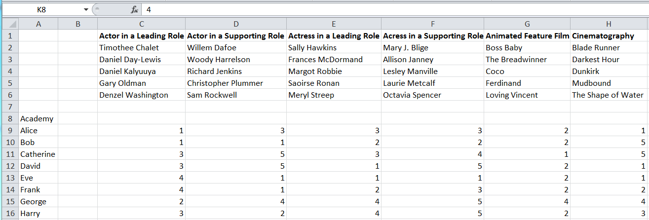
The first thing I do is create a column for each category with the nominees listed underneath it as shown in figure 1. I leave a couple of blank columns to the left so that I can fill in the voters underneath.

Figure 1: Categories and nominees
Then I create a row for each of the voters and fill in the number of their choice to speed up my own "data entry" task a bit. I leave a blank row for the "academy" where I'll record the winners as they're announced throughout the night.

Figure 2: Voters and selections
Now, of course, inputting numbers rather than full text strings saves time and eliminates potential errors,
but isn't very helpful to look at, so I create a second set of rows underneath the first and copy the
formula =INDEX(C$2:C$6,C8) into each of the new cells. The $2 $6
syntax ensures that the rows don't change as the formula is replicated throughout the cells.
In my actual spreadsheet, the rows started further down because there are 10 best picture nominees; I removed the blank rows here because they're distracting.

Figure 3: Actual values
One thing that's sort of annoying is that, since the Academy selections haven't been announced yet, I
see #VALUE! across the top line, since those refer to blank cells in the upper rows. I
fix this by changing the formula to include an "if guard": =IF(C8,INDEX(C$2:C$6,C8),"-").

Figure 4: Cosmetic clean up
Now, as the night goes on, I'll input the actual winners as they're announced into the top row. But...
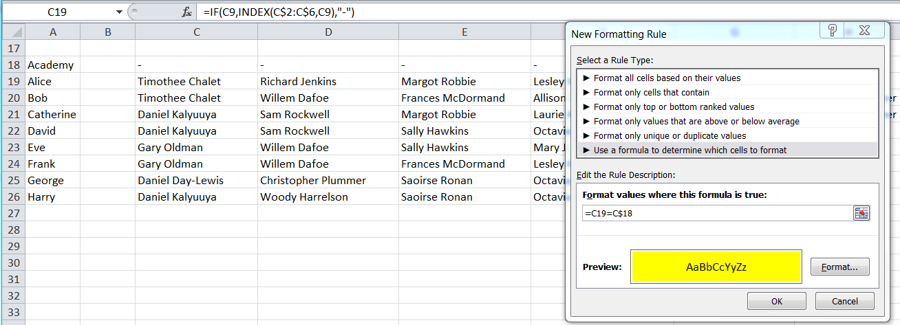
I still have to look to see who actually got which answers right, and how many. To help with the first
problem, I take advantage of Excel's conditional highlighting. I highlight all of the cells that contain
contestant's answers and select "Conditional Formatting" -> "New Rule". I click "Use a formula to
determine which cells to format" and use the formula =C19=C$18 (again using the $
syntax to ensure that, as the cell is replicated through the sheet, the row of the target stays in place).

Figure 5: Highlight the winners
Now, as the winners are announced throughout the night, I fill in the "academy" row and the cells for everybody who predicted correctly light up as in Figure 6.

Figure 6: Track winners as they're announced
I can actually tell at a glance now who's winning as the categories are announced, but I can get Excel
to automatically track that for me, too. What I did was to create yet another copy of the contestants rows and
create a formula in the corresponding cells =IF(C19=C$18,1,0); effectively duplicating the
highlighting logic but as a number so that they can easily be summed in the B column using
=SUM(C28:AA28).

Figure 7: Count winners
Still, it kind of bugged me that I had to copy the list of contestants now three times in various places;
the first instance appears to be unavoidable unless I want to actually type in the text values of
everybody's entries (you can almost do this with a custom cell rule formula, but there doesn't appear to
be a way to key this off of a set of other cells such as with the INDEX function), but
do I need to count cells? I found a sort of complex VBA function for counting the highlighted cells
here,
but actually no VBA is needed. I wish I could take credit for having figured this one out, but
this guy documents how
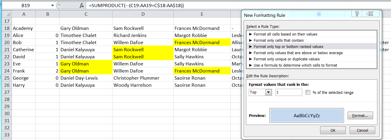
you can effectively convert my IF function from figure 7 into an "in-place" array and sum it
directly using the formula =SUMPRODUCT(--(C19:AA19=C$18:AA$18)). Now I can count the winners
right there in place, and even highlight the current winner as the night goes on.

Figure 8: Count winners without using a special counting area
What he's doing here is creating an array of (FALSE;FALSE;TRUE) entries from the formula,
converting that to 1's and 0's using the -- construct and then adding them all up.
The SUM function doesn't work here because it wants a range of cells rather than an Excel
array; SUMPRODUCT is designed specifically to work with arrays rather than
ranges.
I can even highlight the winners using another conditional formatting rule as show below.

Figure 9: Highlight current winner (or winners)
It's sort of nerdy, but it's a fun way to spend Oscar's night.
Yes, my wife won again this year. I swear we're not cheating. We gave the prize to the second place winner.
Add a comment:
Completely off-topic or spam comments will be removed at the discretion of the moderator.
You may preserve formatting (e.g. a code sample) by indenting with four spaces preceding the formatted line(s)

